Rate Graphs and Orders
This lesson covers:
- Designing experiments to determine the rate equation
- The initial rates method and clock reactions
- Continuous monitoring methods and colorimetry
- Interpreting rate-concentration graphs
- Calculating rate constants from half-life data
Performing rate experiments to determine reaction orders
To determine the reaction order with respect to the concentration of a specific reactant, you can use two main methods:
- Initial rates method - This involves measuring how the initial rate changes when you alter the initial concentration of the reactant in question.
- Continuous monitoring - This involves tracking the change in concentration of the reactant over time and plotting a rate-concentration graph.
In both strategies, ensure that the concentrations of any other reactants remain substantially constant (in large excess) throughout the experiment. This approach helps ensure that any observed changes in rate are solely due to the reactant being studied.
Using the initial rates method to work out rate equations
The initial rate of a reaction refers to the rate at the very beginning of the reaction (time = 0) and is found by calculating the gradient of the tangent to the concentration-time graph at t = 0.

The steps involved in the initial rates method are:
- Perform the reaction several times, each time changing the initial concentration of one reactant while keeping the others constant.
- Calculate the initial rate from the concentration-time data for each experiment.
- Analyse how the initial rates change with varying initial concentrations to deduce the order of the reaction with respect to each reactant.
- Use these findings to assemble the overall rate equation.
Worked example 1 - Determining the rate equation using initial rates
Consider the reaction below, carried out at a constant temperature.
2NO(g) + O2(g) ➔ 2NO2(g)
| Experiment | [NO] (mol dm-3) | [O2] (mol dm-3) | Initial rate (mol dm-3 s-1) |
|---|---|---|---|
| 1 | 0.05 | 0.05 | 0.020 |
| 2 | 0.10 | 0.05 | 0.080 |
| 3 | 0.05 | 0.10 | 0.040 |
Determine the rate equation for this reaction.
Step 1: Analyse NO concentration change
Between experiments 1 and 2, the concentration of [NO] doubles while [O2] remains constant, and the rate quadruples. This suggests the reaction is second order with respect to [NO].
Step 2: Analyse O2 concentration change
Between experiments 1 and 3, doubling the concentration of [O2] while keeping [NO] constant doubles the rate, indicating first-order dependence on [O2].
Step 3: Write the rate equation
rate = k[NO]2[O2]
Worked example 2 - Calculating the rate constant using initial rates
Using the same reaction and data from the previous worked example 1, calculate the rate constant (k), including its units.
Step 1: Rearrange rate equation
First, rearrange the rate equation to solve for k.
k =[NO]2[O2]rate
Step 2: Substitution and correct evaluation
Substitute values from one of the experiments into the equation to find k. For example, substituting values from experiment 1:
k =(0.05)2×0.050.020=160
Step 3: Determine the units
Given that the rate is expressed in mol dm-3 s-1 and the concentration cubed in (mol dm-3)3, solving for k in the equation results in units of mol-2 dm6 s-1.
Therefore the rate constant for the reaction above is 160 mol-2 dm6 s-1.
Simplifying initial rate experiments with clock reactions
Clock reactions offer an easier way to estimate initial rates, avoiding continuous measurements.
In a clock reaction:
- The time taken to produce a fixed amount of product is measured as the initial concentrations of reactants are varied.
- A clear observable change, such as a colour change, signals the endpoint of the reaction.
- The faster the clock reaction finishes, the higher the initial rate.
For this method to be valid, it is assumed that:
- The reactant concentrations do not change appreciably over the timescale of the experiment.
- The temperature remains constant.
If the reaction has not progressed too far by the endpoint, the rate can be assumed to be approximately constant and equal to the initial rate. The initial rate is inversely proportional to time taken for the observerable change to occur.
The iodine clock reaction
The classic example of a clock reaction is the iodine clock:
H2O2(aq) + 2I-(aq) + 2H+(aq) ➔ 2H2O(l) + I2(aq)
A small quantity of sodium thiosulfate and starch indicator is added to an excess of hydrogen peroxide and acidified iodide.
The thiosulfate rapidly consumes any iodine produced:
2S2O32-(aq) + I2(aq) ➔ S4O62-(aq) + 2I-(aq)
Initially, all iodine generated in the first reaction is immediately consumed by the second. However, once the thiosulfate is exhausted, subsequent iodine accumulates, triggering a sudden blue-black colour change due to the starch indicator. This marks the clock reaction endpoint.
By varying the concentration of iodide or hydrogen peroxide while keeping other reactants constant, the time to reach this endpoint will change, reflecting the effect on reaction rate.
Using continuous monitoring methods to work out rate equations
Rather than finding initial rates, some reactions can be continuously monitored as they proceed to completion. The amounts of reactant or product are determined at regular intervals to see how the rate varies over the course of the reaction.
Numerous methods can be used depending on what property changes during the reaction:
- Measuring the volume of gas evolved.
- Measuring the mass loss as a gas escapes.
- Measuring pH changes.
- Using colorimetry to quantify colour changes (see below).
Colorimetry and absorbance
Colorimeters measure the absorbance of a specific wavelength of light by a solution. If the reactant and product have different absorbances at a chosen wavelength, the change in absorbance can be used to monitor the reaction.
Colorimetry involves the following steps:
- Select the appropriate wavelength for monitoring the target species.
- Calibrate the colorimeter using a blank sample (e.g., distilled water) to set the absorbance to zero.
- Withdraw samples from the reaction mixture at fixed time points and measure their absorbance.
To convert absorbance readings into concentrations, a calibration curve must be prepared.
This involves the following steps:
1. Prepare a series of standard solutions with known concentrations of the analyte (reactant or product).
2. Measure the absorbance of each standard solution using the colorimeter.
3. Plot the absorbance values against the corresponding concentrations.
- Fit a trendline to the data points to obtain the calibration curve.
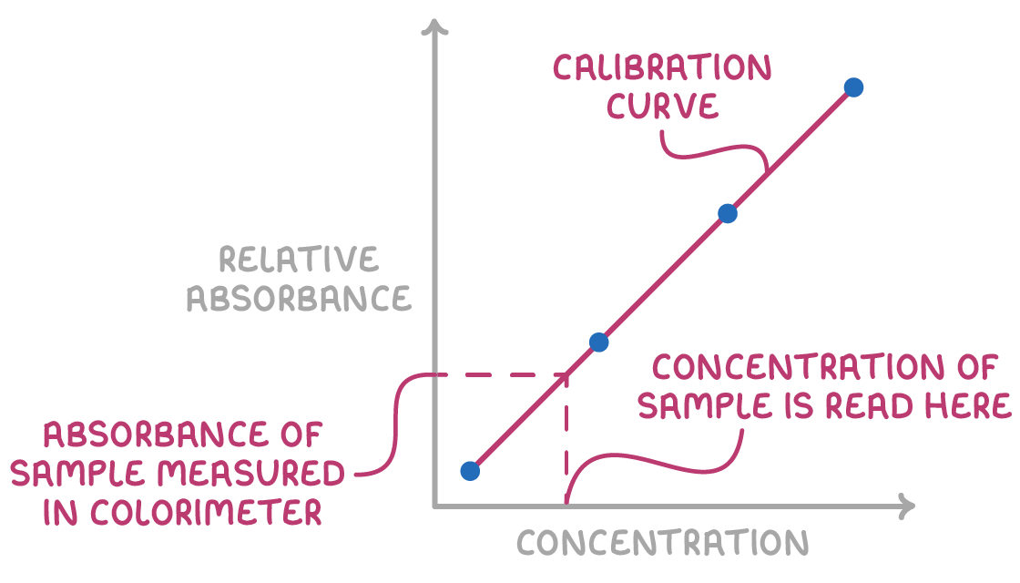
Unknown sample concentrations can then be determined by locating their absorbance on the curve and reading the corresponding concentration from the x-axis.
Determining reaction order from rate-concentration graphs
The shape of a rate-concentration graph can reveal the reaction order with respect to a particular reactant.
To construct a rate-concentration graph from experimental data, follow these steps:
- Begin with a concentration-time graph for the reactant of interest.
- Calculate the rate (gradient) at various points along the concentration-time curve.
- For linear plots, the gradient is constant and can be easily determined.
- For curved plots, draw tangent lines at selected points to determine the gradient at each point.
- Plot the rate (y-axis) against the corresponding concentration (x-axis) for each point.
- Fit a smooth curve or line through the resulting data points.
The shape of the resulting rate-concentration graph reveals the reaction order with respect to the reactant:
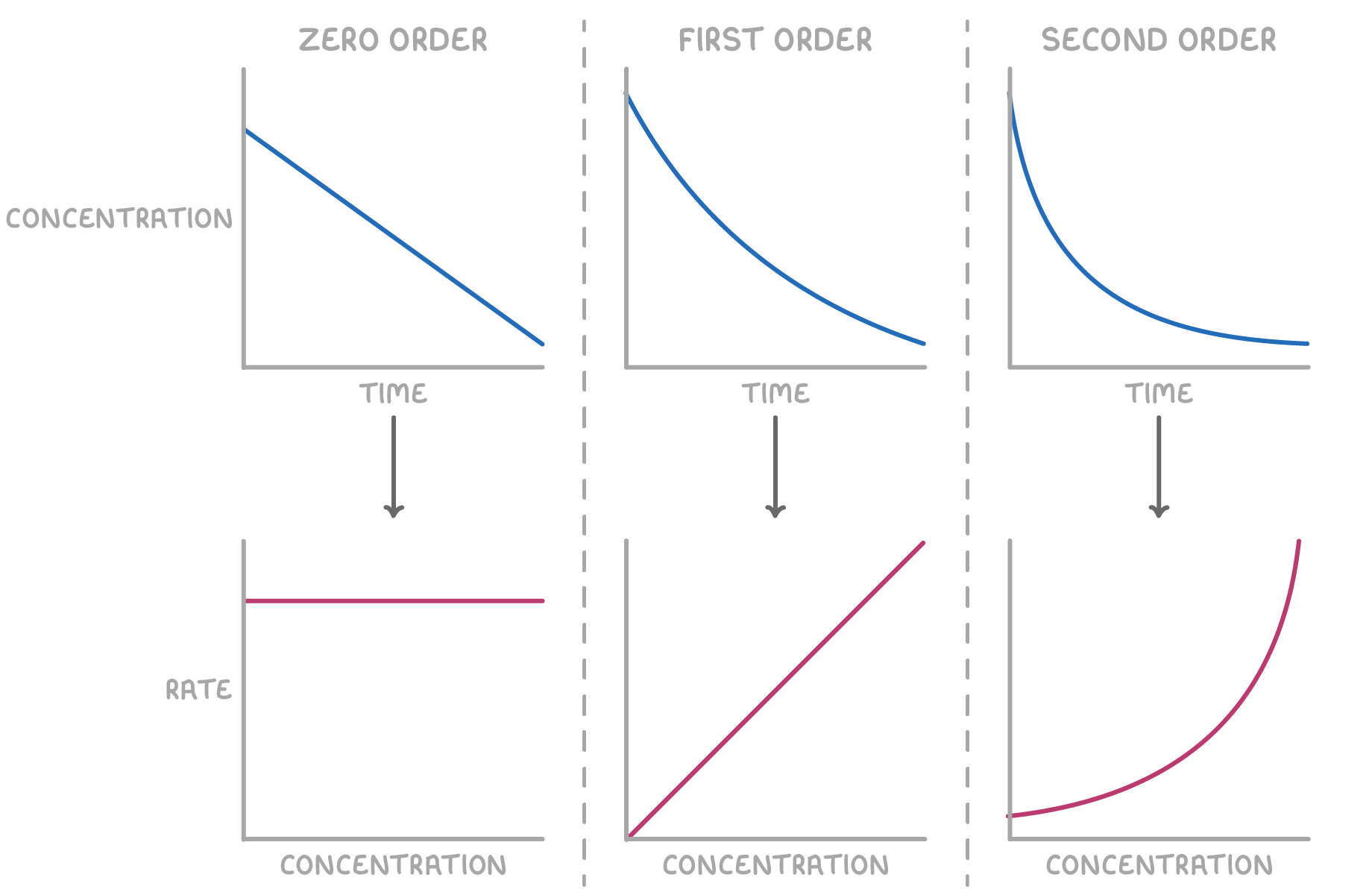
- Zero order - A horizontal line indicates that the reaction rate is independent of the reactant concentration.
The rate equation is: rate = k
- First order - A straight line passing through the origin signifies that the reaction rate is directly proportional to the reactant concentration.
The rate equation is: rate = k[X]
- Second order - A curved plot indicates that the reaction rate is proportional to the square of the reactant concentration.
The rate equation is: rate = k[X]2
In these equations, k represents the rate constant, and [X] denotes the concentration of reactant X.
First order reactions have constant half-lives
The half-life (t21) of a reaction is the time taken for the concentration of a reactant to decrease to half of its initial value.
For first-order reactions:
- The half-life is independent of the initial concentration.
- Each successive half-life is the same duration.
- The half-life can be read directly from the concentration-time graph.
The rate constant (k) of a first-order reaction is related to its half-life (t21) by the equation:
k =t21ln(2)
Worked example 4 - Calculating the rate constant from half-life data
The graph below illustrates the decomposition of hydrogen peroxide.
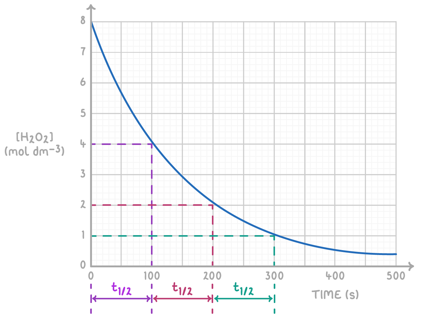
Determine the half-life at different concentration intervals and calculate the rate constant.
Step 1: Determine half-life
Half-life measurements:
- [H2O2] from 8 to 4 mol dm-3: t21 = 100 s
- [H2O2] from 4 to 2 mol dm-3: t21 = 100 s
- [H2O2] from 2 to 1 mol dm-3: t21 = 100 s
The consistent half-life of 100 s, regardless of concentration, confirms that the reaction is first-order with respect to H2O2.
Step 2: Equation
k =t21ln(2)
Step 3: Substitution and correct evaluation
k =100ln(2)=6.93×10⁻³ s−1