Variation

This lesson covers: 

1. The causes of variation
2. Continuous and discontinuous variation
3. Using means and standard deviations to quantify variation

Causes of variation

Variation refers to the differences observed among individuals within any given population. Despite the high degree of similarity, especially in genetically identical organisms such as twins, each individual is distinct.

Variations can arise due to variety of factors.

Genetic factors that cause variation

Genetic variation is variation due to the genes and alleles an individual possesses.

Variations in alleles can lead to different phenotypes, such as the diversity seen in human blood groups.

Sources of genetic variation:

1. Mutations - Changes to genes and chromosomes that may be passed on to the next generation.
2. Meiosis - New combinations of alleles are present in the gametes formed, produced by independent assortment of chromosomes and crossing over between chromatids.
3. Random fertilisation - Random fertilisation of gametes produces new combinations of alleles in a zygote.
4. Random mating

Environmental factors that cause variation

Environmental variation is variation caused by the environment in which an organism lives.

Differences in environmental factors like climate or diet can cause variations among individuals, such as variations in accents or the presence of pierced ears.

Environmental factors that can cause variation include:

1. Light
2. Nutrient and food availability
3. Temperature
4. Rainfall
5. Soil conditions
6. pH

Environmental influences can also affect the way an organism's genes are expressed.

The combined effect of genetic and environmental factors on variation

While genetic makeup sets the potential for variation, environmental conditions can influence the actual outcome, such as with human height.

It is hard to distinguish between the effects of genetic and environmental influences on variation as many genetic and environmental influences combine to produce differences between individual.

Polygenes:

• These are different genes at different loci that all contribute to a particular aspect of phenotype.
• Their individual effects on a phenotype are too small to observe, but they can act together to produce observable variation.
• This combined effect of multiple genes is common in continuous variation.

Continuous and discontinuous variation

Variation may either be continuous or discontinuous.

Continuous variation:

• This is when there are a range of values between two extremes without distinct categories, which produce a spectrum of phenotypes.
• An example is the variation in milk yield among cows.
• Typically affected by both genes and environment.

Discontinuous variation:

• This features clear, distinct categories with no intermediates.
• For instance, human blood types can be classified as A, B, AB, or O.
• Typically caused entirely by genes.

Quantifying variation using means

The mean provides an average value of a sample. Comparing the means of different samples helps identify variation.

For example:

• Mean tree height in sample of woodland A = 30 m.
• Mean tree height in sample of woodland B = 50 m.

This 20 m difference shows variation between the samples, which indicates variation between the actual woodland tree populations.

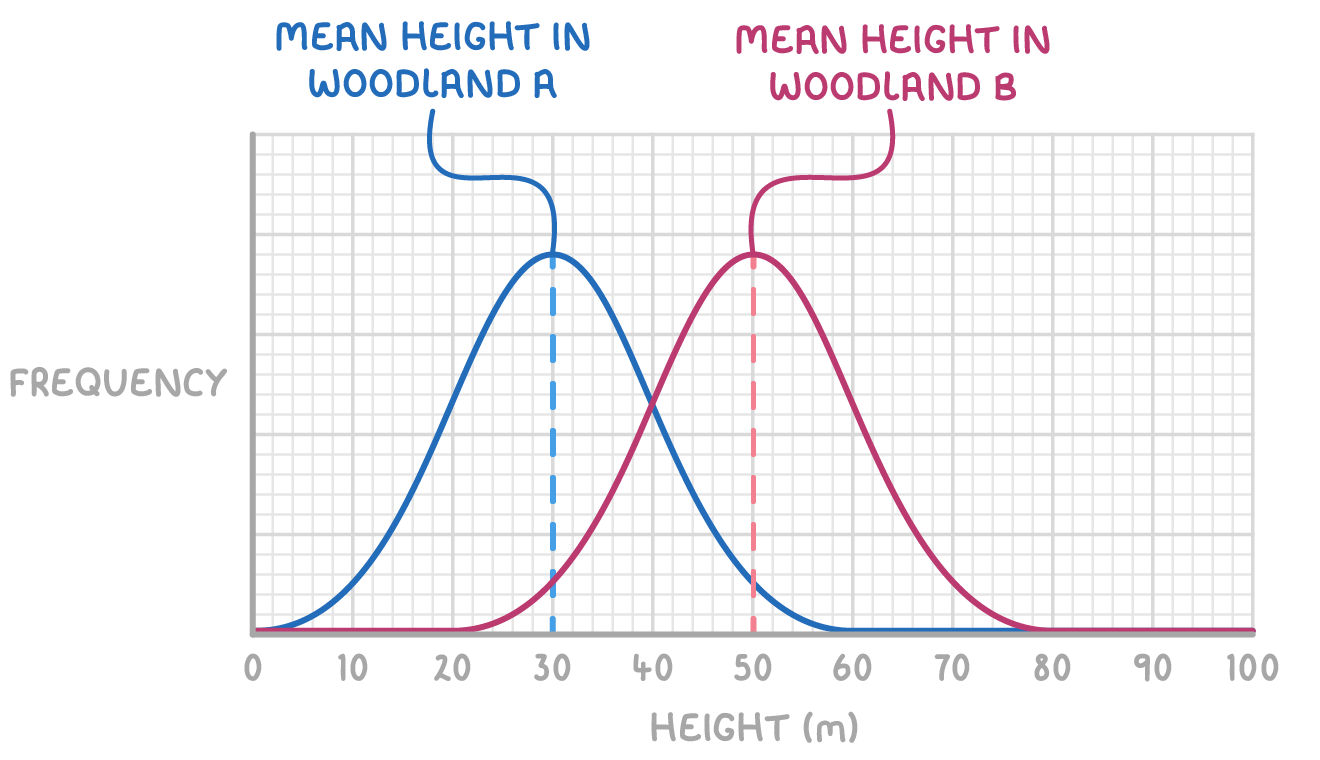
Most samples with values either side of the mean will be normally distributed. A normal distribution curve is bell-shaped and symmetrical around a central mean value, like those shown for woodlands A and B above.

A normal distribution curve will often be produced when plotting a graph for a characteristic that exhibits continuous variation. For instance, in the graph we can see the frequency of trees of different heights in two woodlands, and the range of heights shows continuous variation.

Quantifying variation using standard deviation

The standard deviation measures how spread out the values are from the mean.

What values of standard deviation represent:

• Smaller standard deviation - There are fairly consistent values that are clustered around the mean.
• Larger standard deviation - There are fairly inconsistent values that are widely spread around the mean.

The mean height of woodland A in the example above may be represented as 30 m ± 5 m.

• This means that the mean is 30 and the standard deviation is 5.
• Most (~68%) values lie between 25 m and 35 m.

To calculate the standard deviation, we use the following formula (this will be provided):

standard deviation =√n−1Σ(x−xˉ)2​​

Where:

Σ= the sum of

x = measured value (from the sample)

xˉ= mean value

n = total number of values in the sample

Worked example - Quantifying tree height variation using standard deviation

Calculate the standard deviation of tree heights in a sample from a woodland, given the following data that has been collected for tree heights in metres: 32, 35, 31, 29, 33.

Step 1: Equation

standard deviation =√n−1Σ(x−xˉ)2​​

Step 2: Calculate the mean (xˉ)

xˉ=nsum of all tree heights​

xˉ=532+35+31+29+33​

xˉ=5160​=32

Step 3: Calculate (x−xˉ)2 for each tree height

for each tree height, subtract the mean and square the result

(x1​−xˉ)2=(32−32)2=0

(x2​−xˉ)2=(35−32)2=9

(x3​−xˉ)2=(31−32)2=1

(x4​−xˉ)2=(29−32)2=9

(x5​−xˉ)2=(33−32)2=1

Step 4: Summation and division

sum all squared differences and divide by n−1

Σ(x−xˉ)2=0+9+1+9+1

Σ(x−xˉ)2=20

n−1Σ(x−xˉ)2​=5−120​

n−1Σ(x−xˉ)2​=420​=5

Step 5: Square root

take the square root of this value to get the standard deviation

standard deviation of tree heights in woodland =√5≈2.24 m